|
For starting with deep learning Theano is one of the best Deep learning framework available at present. But its better to use it with the wrapper built over the theano platform to speed up the coding and design testing process. Keras is most suitable wrapper due to its easy to use design and support available online which will help you tackle problem faster if it comes. Anaconda package will be used to install python and python related other dependencies. Advantage of anaconda is that it has all the required packages already so you don't have to install each package individually. Anaconda is open source distribution. The process of installation is as below. 1. Download Anaconda from the link https://www.continuum.io/downloads . You can download any version but python 3.5 version will be recommend. 2. After downloading the shell file, open from terminal and run it from its directory complete the installation process 3. close and reopen the terminal for changes to take place. Then write following command 5. To check if liberaries installed correctly and completely. Open python and import these libraries If the above error massage (ImportError: No module named ‘tensorflow’) is shown then it means actually keras is by default configured for tensorflow backend so if you want to change to teano backend
Go to home directory
{ “image_dim_ordering”: “th”, “backend”: “theano”, “floatx”: “float32”, “epsilon”: 1e-07 }
0 Comments
Recurrent Neural Network: The fundamental feature of a Recurrent Neural Network (RNN) is that the network contains at least one feed-back connection, so the activations can flow round in a loop. That enables the networks to do temporal processing and learn sequences, e.g., perform sequence recognition/reproduction or temporal association/prediction. Recurrent neural network architectures can have many different forms. One common type consists of a standard Multi-Layer Perceptron (MLP) plus added loops. These can exploit the powerful non-linear mapping capabilities of the MLP, and also have some form of memory. Others have more uniform structures, potentially with every neuron connected to all the others, and may also have stochastic activation functions. For simple architectures and deterministic activation functions, learning can be achieved using similar gradient descent procedures to those leading to the back-propagation algorithm for feed-forward networks. In sequential tasks such as natural language and speech processing, there is always dependence of present input data upon the previous applied inputs. Task of RNNs is to find the relationship between current input and the previous applied inputs. In theory RNNs can make use of information sequence of any arbitrarily length, but in practice they are limited to looking back only a few steps. 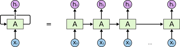 Figure: Basic architecture of Recurrent Neural Networks The above figure shows a RNN being unfolded into a full network. By unfolding we simply mean that we are repeating the same layer structure of network for the complete sequence. Xt is the input at time step t. Xt is a vector of any size N. A is the hidden state at time step t. It’s the “memory” of the network. It is calculated based on the previous hidden state and the input at the current step. Represented by At= f (W Xt +U At-1) Here W and U are weights for input and previous state value input. And f is the non-linearity applied to the sum to generate final cell state. One of the appeals of RNNs is the idea that they might be able to connect previous information to the present task, such as using previous video frames might inform the understanding of the present frame. If RNNs could do this, they’d be extremely useful. Sometimes, we only need to look at recent information to perform the present task. For example, consider a language model trying to predict the next word based on the previous ones. If we are trying to predict the last word in “the clouds are in the sky,” we don’t need any further context – it’s pretty obvious the next word is going to be sky. In such cases, where the gap between the relevant information and the place that it’s needed is small, RNNs can learn to use the past information. In theory, RNNs are absolutely capable of handling such “long-term dependencies.” A human could carefully pick parameters for them to solve toy problems of this form. Sadly, in practice, RNNs don’t seem to be able to learn them. Long Short Term Memory networks: Normally called as LSTMs, they are a special kind of RNN, capable of learning long-term dependencies. They work tremendously well on a large variety of problems, and are now widely used. LSTMs are explicitly designed to avoid the long-term dependency problem. Remembering information for long periods of time is practically their default behavior. All recurrent neural networks have the form of a chain of repeating modules of neural network. In standard RNNs, this repeating module will have a very simple structure, such as a single tanh layer. In all traditional recurrent neural network, during the gradient back-propagation phase, the gradient signal can end up being multiplied a large number of times (as many as the number of time steps) by the weight matrix associated with the connections between the neurons of the recurrent hidden layer. This means that, the magnitude of weights in the transition matrix can have a strong impact on the learning process. If the weights in this matrix are small (or, more formally, if the leading eigenvalue of the weight matrix is smaller than 1.0), it can lead to a situation called vanishing gradients where the gradient signal gets so small that learning either becomes very slow or stops working altogether. It can also make more difficult the task of learning long-term dependencies in the data. Conversely, if the weights in this matrix are large (or, again, more formally, if the leading eigenvalue of the weight matrix is larger than 1.0), it can lead to a situation where the gradient signal is so large that it can cause learning to diverge. This is often referred to as exploding gradients. These issues are the main motivation behind the LSTM model which introduces a new structure called a memory cell . A memory cell is composed of four main elements: an input gate, a neuron with a self-recurrent connection (a connection to itself), a forget gate and an output gate. The self-recurrent connection has a weight of 1.0 and ensures that, barring any outside interference, the state of a memory cell can remain constant from one time step to another. The gates serve to modulate the interactions between the memory cell itself and its environment. The input gate can allow incoming signal to alter the state of the memory cell or block it. On the other hand, the output gate can allow the state of the memory cell to have an effect on other neurons or prevent it. Finally, the forget gate can modulate the memory cell’s self-recurrent connection, allowing the cell to remember or forget its previous state, as needed. 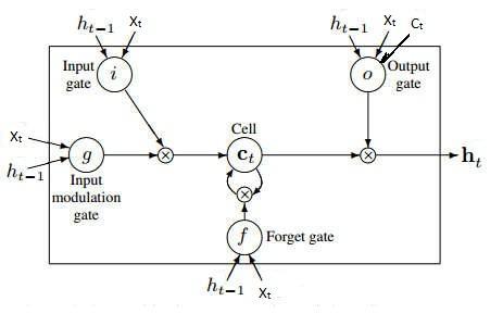 Figure: A single cell of LSTM Network
The three gates in LSTM are input gate [i], forget gate [f] and output gate [o]. The input to be updated in cell at current time step is [g]. all of these gates and update signal are dependent on previous hidden state and the current input of the cell as per principle of recurrent nets. So, it = f ( Wi Xt + Ui ht-1 + bi ) gt = tanh ( Wc Xt + Uc ht-1 + bc ) ft = f ( Wf Xt + Uf ht-1 + bf ) Now value to be updated in cell can be calculated using these three equations as Ct = it .gt + ft .Ct-1 The output of this LSTM cell can be generated by using current cell state, current input and previous output. all these three signals are used to control output gate. According to the state of output gate, cell state is passed through the tanh function, just to keep output near zero and one. Ot = f ( Wo Xt + Uo ht-1 + Vo Ct + bo ) ht = Ot . tanh( Ct) This LSTM cell is organised in same order as mnetioned in RNN architecture and size of the network depends on sequential dependency or relation between data. Convolutional neural networks (CNNs) are a specialized kind of neural network for processing data which has spatial correlation between the neighborhood data points which is also called as grid-like topology. Examples of the data include time-series data, which can be thought of as a 1D grid taking samples at regular time intervals, and image data, which can be thought of as a 2D grid of pixels. Convolutional networks have been tremendously successful in practical applications. The name “convolutional neural network” indicates that the network employs a mathematical operation called convolution. Convolution is a specialized kind of linear operation. Convolutional networks are simply neural networks that use convolution in place of general matrix multiplication in at least one of their layers. Convolution leverages three important ideas that can help improve a machine learning system:
Moreover, convolution provides a means for working with inputs of variable size. Convolutional Neural Networks take advantage of the fact that the input consists of images and they constrain the architecture in a more sensible way. In particular, unlike a regular Neural Network, the layers of a CNN have neurons arranged in 3 dimensions: width, height, depth. Word depth here refers to the third dimension of an activation volume, not to the depth of a full Neural Network, which can refer to the total number of layers in a network. For example, the input images in CIFAR-10 are an input volume of activations, and the volume has dimensions 32x32x3 (width, height, depth respectively). The neurons in a layer will only be connected to a small region of the layer before it, instead of all of the neurons in a fully-connected manner. Moreover, the final output layer would for CIFAR-10 have dimensions 1x1x10, because by the end of the CNN architecture we will reduce the full image into a single vector of class scores, arranged along the depth dimension. 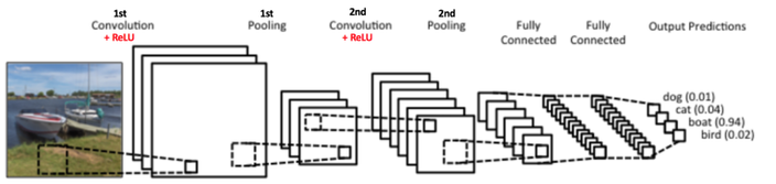 Figure: Basic architecture of Convolutional Neural Networks A simple CNN is a sequence of layers, and every layer of a CNN transforms one volume of activations to another through a differentiable function. We use four main types of layers to build CNN architectures: Convolutional Layer, Activation Layer, Pooling Layer, and Fully-Connected Layer. We will stack these layers to form a full CNN architecture. The detailed description of these layers is as follows: INPUT LAYER- the input layer is the input image given to the network and is represented in form of [M*N*D] which will hold the raw pixel values of the image. Here M and N represent the hight and width of the image and D is the color dimetions i.e. if image is gray then D=1 and if its RGB image then D=3. CONVOLUTIONAL LAYER- This layer will compute the output of neurons that are connected to local regions in the input, each computing a dot product between their weights and a small region they are connected to in the input volume. If we are using 10 convolutional filters at first layer then output of the first layer will be [M*N*F]. where F is the number of the filters and size of each filter is denoted by [x*y*D]. where D is third dimention of image and x and y are the size of the filter. Generally we take x=y=3. 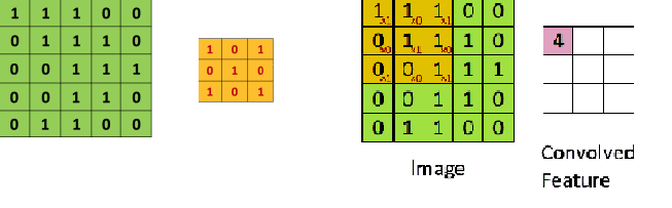 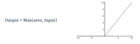 Figure: Convolution operation Stride: Stride is the number of pixels by which we slide our filter matrix over the input matrix. When the stride is 1 then we move the filters one pixel at a time. When the stride is 2, then the filters jump 2 pixels at a time as we slide them around. Having a larger stride will produce smaller feature maps. Zero-padding: Sometimes, it is convenient to pad the input matrix with zeros around the border, so that we can apply the filter to bordering elements of our input image matrix. A nice feature of zero padding is that it allows us to control the size of the feature maps. Adding zero-padding is also called wide convolution, and not using zero-padding would be a narrow convolution. ACTIVATION LAYER- the activation layer comes after each convolutional layer and it represents the non linear function used to control the output of each layer. It can be related to the firing mechanism of the biological neurons. This nonlinearity decides which part of the input signal is actually going to contribute into the class label. The location in input image for which particular receptive field fires denotes the importance of that area into actual label. There are three main types of non-linearities used in CNNs which are Rectified Linear Unit (RELU), Tanh and Sigmoid. Figure: Rectified Linear Unit (ReLU) Commonly used ReLU is an element wise operation (applied per pixel) and replaces all negative pixel values in the feature map by zero. The purpose of ReLU is to introduce non-linearity in our ConvNet, since most of the real-world data we would want our ConvNet to learn would be non-linear (Convolution is a linear operation – element wise matrix multiplication and addition, so we account for non-linearity by introducing a non-linear function like ReLU). 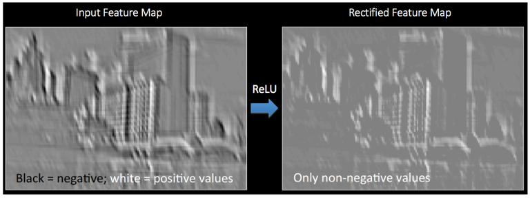 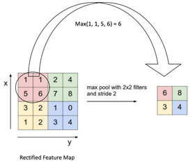 Figure: Feature map of CNN before and after passing through ReLU
POOLING LAYER- Spatial Pooling also called sub-sampling or down-sampling, reduces the dimensionality of each feature map but retains the most important information. Spatial Pooling can be of different types: Max, Average, Sum etc. In case of Max Pooling, we define a spatial neighborhood (for example, a 2×2 window) and take the largest element from the rectified feature map within that window. Instead of taking the largest element we could also take the average (Average Pooling) or sum of all elements in that window. In practice, Max Pooling has been shown to work better. Figure: Max pooling operation Advantages of pooling are: • Makes the input representations (feature dimension) smaller and more manageable • Reduces the number of parameters and computations in the network, therefore, controlling overfitting. • Makes the network invariant to small transformations, distortions and translations in the input image (a small distortion in input will not change the output of Pooling – since we take the maximum / average value in a local neighborhood). • Helps us arrive at an almost scale invariant representation of our image. This is very powerful since we can detect objects in an image no matter where they are located. It is important to understand that the layers discussed above are the basic building blocks of any CNN. In the image, we have two sets of Convolution, ReLU & Pooling layers – the 2nd Convolution layer performs convolution on the output of the first Pooling Layer using six filters to produce a total of six feature maps. ReLU is then applied individually on all of these six feature maps. We then perform Max Pooling operation separately on each of the six rectified feature maps. Together these layers extract the useful features from the images, introduce non-linearity in our network and reduce feature dimension while aiming to make the features invariant to scale and translation.The output of the 2nd Pooling Layer acts as an input to the Fully Connected Layer, which we will discuss in the next section. FULLY CONNECTED LAYER- The Fully Connected layer is a traditional Multi Layer Perceptron that uses a softmax activation function in the output layer (or sometimes other classifiers like SVM). The term “Fully Connected” implies that every neuron in the previous layer is connected to every neuron on the next layer. The output from the convolutional and pooling layers represent high-level features of the input image. The purpose of the Fully Connected layer is to use these features for classifying the input image into various classes based on the training dataset. Apart from classification, adding a fully-connected layer is also a cheap way of learning non-linear combinations of these features. Most of the features from convolutional and pooling layers may be good for the classification task, but combinations of those features might be even better. The sum of output probabilities from the Fully Connected Layer is 1. This is ensured by using the Sofmax, the activation function in the output layer of the Fully Connected Layer. The Softmax function takes a vector of arbitrary real-valued scores and squashes it to a vector of values between zero and one that sum to one. |
AuthorMy Name is Vivek Singh Bawa. I am a research scholar of deep learning and compute vision. CategoriesArchives |
 RSS Feed
